Classification

MultiLayerNetwork linear classification example.

from miml import datasets
from miml.deep_learning import Network
from miml.deep_learning import Dense, Output

fn = os.path.join(datasets.get_data_home(), 'classification',
    'linear_data_train.csv')
df = DataFrame.read_table(fn, delimiter=',', header=None, names=['x1','x2'],
    format='%2f', index_col=0)

X = df.values
y = array(df.index.data)

model = Network(seed=123, weight_init='xavier', learn_rate=0.01, momentum=0.9)
model.add(Dense(nin=2, nout=20, activation='relu'))
model.add(Output(loss='negativeloglikelihood', nin=20, nout=2, activation='softmax'))
model.compile()
for i in range(30):
    print 'Epoch: %i' % (i + 1)
    si = 0
    while si < len(X):
        model.fit(X[si:si+50], y[si:si+50])
        si += 50

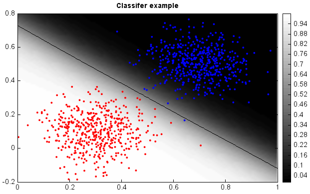
# Plot the decision boundary. For that, we will assign a color to each
# point in the mesh [x_min, x_max]x[y_min, y_max].
x_min, x_max = 0., 1.
y_min, y_max = -0.2, 0.8
n = 100  # size in the mesh
xx, yy = np.meshgrid(np.linspace(x_min, x_max, n),
                     np.linspace(y_min, y_max, n))
data = np.vstack((xx.flatten(), yy.flatten())).T
z = model.predict(data)

# Put the result into a color plot
Z = z[:,0].reshape(xx.shape)

#Plot
# Create color maps
cmap_light = ['#FFAAAA', '#AAAAFF']
cmap_bold = ['#FF0000', '#0000FF']
gg = imshow(xx[0,:], yy[:,0], Z, 40, cmap='MPL_gist_gray', interpolation='bilinear')
# Plot also the training points
plt.scatter(X[:, 0], X[:, 1], c=y,
    edgecolor=None, s=4, levels=[0,1], colors=cmap_bold)
plt.contour(xx[0,:], yy[:,0], Z, [0.5], color='k', smooth=False)
colorbar(gg)
plt.xlim(xx.min(), xx.max())
plt.ylim(yy.min(), yy.max())
plt.title("Classifer example")