MeteoInfo 1.4.6 was released (2017-7-31)

Several 3D plot function were added in Axes3D class, including plot(), scatter(), contour(), contourf(), imshow(), plot_surface(), plot_wireframe() and plot_layer.

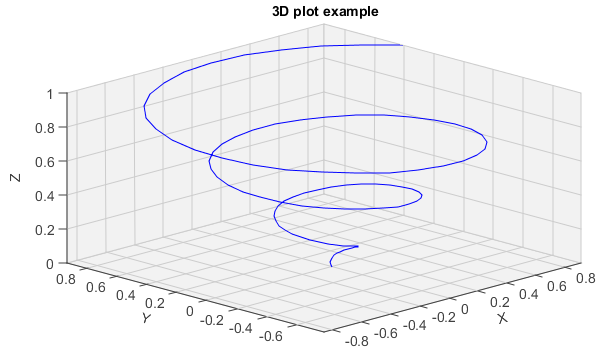
Line plots:

z = linspace(0, 1, 100)
x = z * np.sin(20 * z)
y = z * np.cos(20 * z)

#Plot
ax = axes3d()
ax.plot(x, y, z, '-b')
title('3D plot example')

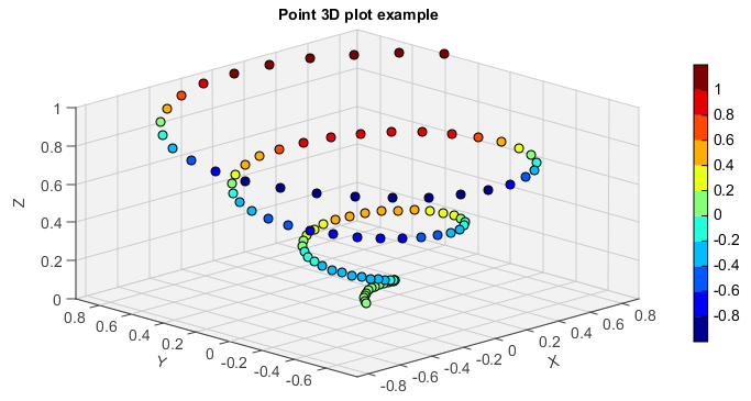
Scatter plots:

z = linspace(0, 1, 100)
x = z * np.sin(20 * z)
y = z * np.cos(20 * z)
c = x + y

#Plot
ax = axes3d()
points = ax.scatter(x, y, z, c=c)
colorbar(points,shrink=0.8)
title('Point 3D plot example')

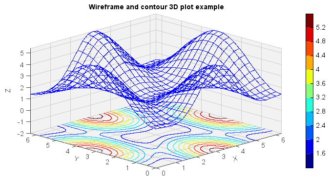
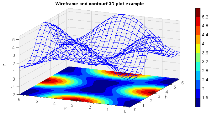
Wireframe and contour plots:

alpha = 0.7
phi_ext = 2 * pi * 0.5
N = 25
x1 = linspace(0, 2*pi, N)
y1 = linspace(0, 2*pi, N)
x,y = meshgrid(x1, y1)
z = 2 + alpha - 2 * cos(y) * cos(x) - alpha * cos(phi_ext - 2 * y)
z = z.T

#Plot
ax = axes3d()
lines = ax.contour(x1, y1, z, 10, offset=-2)
ax.plot_wireframe(x, y, z, color='b')
colorbar(lines)
title('Wireframe and contour 3D plot example')

Wireframe and contourf plots:

alpha = 0.7
phi_ext = 2 * pi * 0.5
N = 25
x1 = linspace(0, 2*pi, N)
y1 = linspace(0, 2*pi, N)
x,y = meshgrid(x1, y1)
z = 2 + alpha - 2 * cos(y) * cos(x) - alpha * cos(phi_ext - 2 * y)
z = z.T

#Plot
ax = axes3d()
lines = ax.contourf(x1, y1, z, 10, offset=-2)
ax.plot_wireframe(x, y, z, color='b')
colorbar(lines)
title('Wireframe and contourf 3D plot example')

Surface plots:

alpha = 0.7
phi_ext = 2 * pi * 0.5
x = linspace(0, 2*pi, 100)
y = linspace(0, 2*pi, 100)
x,y = meshgrid(x, y)
z = 2 + alpha - 2 * cos(y) * cos(x) - alpha * cos(phi_ext - 2 * y)
z = z.T

#Plot
ax = axes3d()
ls = ax.plot_surface(x, y, z, 20, edge=False)
colorbar(ls,shrink=0.8)
title('Surface 3D plot example')

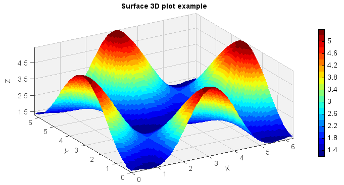
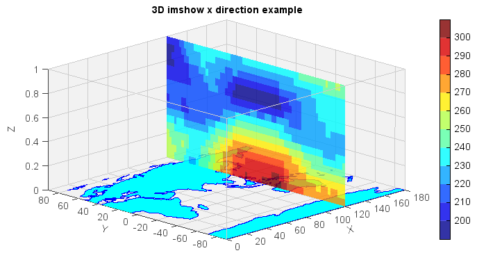
Image plots:

fn = 'D:/Temp/nc/air_clm.nc'
f = addfile(fn)
ps = f['aveair'][0,:,:,'120']
yy = linspace(0, 1., ps.shape[0])
ps.setdimvalue(0, yy)

#Map layer
layer = shaperead('D:/Temp/map/110m-land.shp')

#Plot
ax = axes3d(bbox=True)
ax.plot_layer(layer, color='c', edgecolor='b')
ls = ax.imshow(ps, 10, offset=120, zdir='x', alpha=0.8)
colorbar(ls)
zlim(0, 1)
xlim(0, 180)
title('3D imshow x direction example')

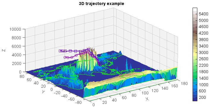
Trajectory plots:

#Open trajectory data and get trajectory layer
fn = 'D:/Temp/HYSPLIT/traj_20131211_00'
f = addfile_hytraj(fn)
tlayer = f.trajlayer()
stlayer = f.trajsplayer()

#Map layer
layer = shaperead('D:/Temp/map/110m-land.shp')

#Relief data
fn = 'D:/Temp/nc/elev.0.25-deg.nc'
f = addfile(fn)
elev = f['data'][0,::8,::8]
elev = elev[:,'0:180']
elev[elev<0] = 0

#Plot
ax = axes3d()
ls = ax.plot_surface(elev, 20, cmap='MPL_terrain', edge=False)
ax.plot_layer(layer, edgecolor='g')
ax.plot_layer(tlayer)
ax.plot_layer(stlayer, fill=False)
zlim(0, 10000)
xlim(0, 180)
colorbar(ls)
title('3D trajectory example')