griddata
- mipylib.numeric.interpolate.griddata(points, values, xi=None, **kwargs)
Interpolate scattered data to grid data.
- Parameters:
points – (list) The list contains x and y coordinate arrays of the scattered data.
values – (array_like) The scattered data array.
xi – (list) The list contains x and y coordinate arrays of the grid data. Default is
None, the grid x and y coordinate size were both 500.method – (string) The interpolation method. [idw | cressman | nearest | inside_mean | inside_min | inside_max | inside_sum | inside_count | surface | barnes | kriging]
fill_value – (float) Fill value, Default is
nan.pointnum – (int) Only used for ‘idw’ method. The number of the points to be used for each grid value interpolation.
radius – (float) Used for ‘idw’, ‘cressman’ and ‘neareast’ methods. The searching raduis. Default is
Nonein ‘idw’ method, means no raduis was used. Default is[10, 7, 4, 2, 1]in cressman method.convexhull – (boolean) If the convexhull will be used to mask result grid data. Default is
False.
- Returns:
(array) Interpolated grid data (2-D array)
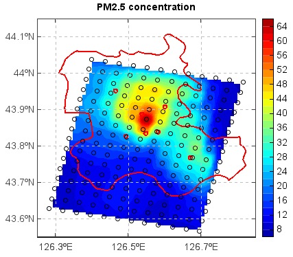
IDW method example
f = addfile('D:/temp/nc/out.20140421_20140421_JL3KMmeic.nc')
data = f['PM25']
data = data[15,1,:,:]
lon = f['lon'][:,:]
lat = f['lat'][:,:]
#Interpolate data to grid
lon1 = linspace(lon.min(), lon.max(), lon.dimlen(1)*5)
lat1 = linspace(lat.min(), lat.max(), lat.dimlen(0)*5)
data1 = griddata((lon, lat), data, xi=(lon1, lat1), method='idw', convexhull=True)[0]
lon_g,lat_g = meshgrid(lon1, lat1)
#Plot
axesm()
mlayer = shaperead('D:/temp/map/jilin.shp')
geoshow(mlayer, edgecolor='r', size=2)
layer = contourfm(lon1, lat1, data1, 20)
scatterm(lon, lat, data, 20, fill=False)
colorbar(layer)
xlim(126.25,126.85)
ylim(43.55,44.15)
grid(True)
title('PM2.5 concentration')
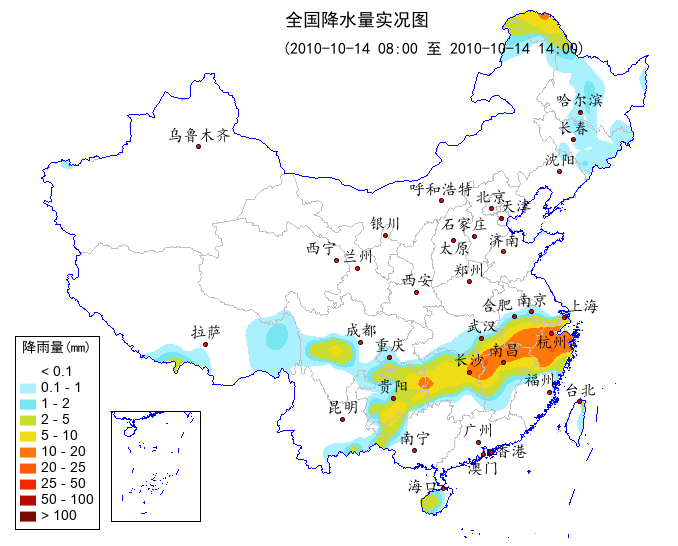
Kriging method example
fn = os.path.join(migl.get_sample_folder(), 'MICAPS', '10101414.000')
f = addfile_micaps(fn)
pr = f['Precipitation6h'][:]
lon = f['Longitude'][:]
lat = f['Latitude'][:]

mask_rect = geolib.polygon([72,72,136,136], [16,55,55,16])
pr,lon,lat = geolib.rmaskout(pr, lon, lat, mask_rect)
idx = where(pr != nan)
pr = pr[idx]
lon = lon[idx]
lat = lat[idx]

#griddata function - interpolate
x = arange(75, 135, 0.5)
y = arange(18, 55, 0.5)
prg = griddata((lon, lat), pr, xi=(x, y), method='kriging')[0]

#Plot
figure(figsize=[700,550], newfig=False)
proj = projinfo(proj='lcc', lon_0=105, lat_1=25, lat_2=47)
axesm(projinfo=proj, position=[0.01, 0.01, 0.99, 0.99], axison=False, gridlabel=False, frameon=False)
geoshow('cn_province', edgecolor='lightgray')
bou1_layer = geoshow('cn_border', facecolor=(0,0,255))
city_layer = geoshow('cn_cities', facecolor='r', size=4)
city_layer.addlabels('NAME', fontname=u'楷体', fontsize=16, yoffset=15, avoidcoll=False)
china_layer = geoshow('china', visible=False)
city_layer.movelabel(u'西宁', -15)
city_layer.movelabel(u'海口', -20, -10)
city_layer.movelabel(u'澳门', 0, -25)
city_layer.movelabel(u'香港', 20, -10)
city_layer.movelabel(u'福州', -10)
city_layer.movelabel(u'合肥', -18)
city_layer.movelabel(u'杭州', 0, -20)
city_layer.movelabel(u'上海', 18)
city_layer.movelabel(u'太原', 0, -20)
city_layer.movelabel(u'天津', 15)
city_layer.movelabel(u'石家庄', -10)
levs = [0.1, 1, 2, 5, 10, 20, 25, 50, 100]
cols = [(255,255,255),(170,240,255),(120,230,240),(200,220,50),(240,220,20),(255,120,10),(255,90,10), \
    (240,40,0),(180,10,0),(120,10,0)]
layer = contourf(x, y, prg, levs, colors=cols)
masklayer(china_layer, [layer])
legend(layer, loc='lower left', frameon=True, title=u'降雨量(mm)', titlefontname=u'黑体')
axism([79, 128, 14, 53])
text(95, 53, u'全国降水量实况图', fontname=u'黑体', fontsize=18)
text(95, 51, u'(2010-10-14 08:00 至 2010-10-14 14:00)', fontname=u'黑体', fontsize=16)

#Add south China Sea
sc_layer = bou1_layer.clone()
axesm(position=[0.15,0.05,0.15,0.2], axison=False, frameon=True)
geoshow(sc_layer, facecolor=(0,0,255))
xlim(106, 123)
ylim(2, 23)