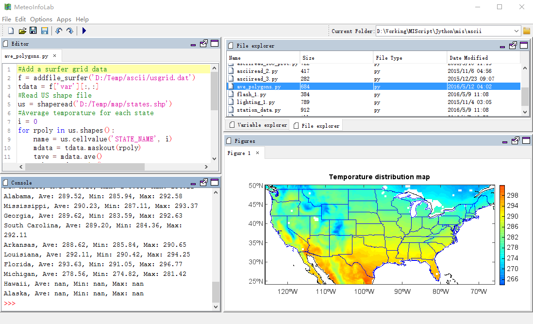
Average data in each polygon
Array data can be masked using polygons, then statistical values of the polygons can be obtained using the masked array. Below script will get average, min, max temporature of each state in US.
#Add a surfer grid data
f = addfile_surfer('D:/Temp/ascii/usgrid.dat')
tdata = f['var'][:,:]
#Read US shape file
us = shaperead('D:/Temp/map/states.shp')
#Average temporature for each state
i = 0
for rpoly in us.shapes():
    name = us.cellvalue('STATE_NAME', i)
    mdata = tdata.maskout(rpoly)
    tave = mdata.ave()
    tmin = mdata.min()
    tmax = mdata.max()
    print name + ', Ave: %.2f, Min: %.2f, Max: %.2f' %(tave, tmin, tmax)
    i += 1

#Plot
axesm()
geoshow('country')
geoshow(us, edgecolor=[0,0,255])
layer = contourf(tdata,20)
title('Temporature distribution map')
colorbar(layer)
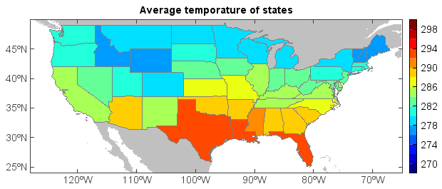
Layer read from shape file can add field and associated values, so we can set the average temporature to each state and plot using graduated colors.
#Read temporature data from a surfer grid data
f = addfile_surfer('D:/Temp/ascii/usgrid.dat')
tdata = f['var'][:,:]

#Read US states layer from shape file
us = shaperead('D:/Temp/map/states.shp')

#Add temp field
us.addfield('temp', 'float')

#Average temporature for each state and add to the temp field
for i in range(us.shapenum()):
    rpoly = us.shapes()[i]
    mdata = tdata.maskout(rpoly)
    tave = mdata.ave()
    us.setcellvalue('temp', i, tave)

#Plot
axesm()
geoshow('country', facecolor='lightgray', edge=False)
levs = arange(270, 300, 2)
cols = makecolors(len(levs)+1)
ls = makesymbolspec('polygon', field='temp', levels=levs, colors=cols,
    edge=True, edgecolor='gray')
geoshow(us, symbolspec=ls)
xlim(-128, -65)
ylim(24, 50)
title('Average temporature of states')
colorbar(us)