Baroclinic Potential Vorticity Analysis

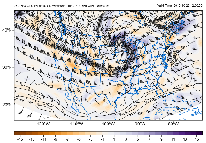
Classic baroclinic potential vorticity plot at 250 hPa using GFS analysis file.

This example uses example data from the GFS analysis for 12 UTC 31 October 2016 and calculate the baroclinic potential vorticity, divergence and wind speed with geographic plotting for a CONUS view of the 250-hPa surface with divergence and wind barbs.

fn = 'D:/Temp/nc/GFS_20101026_1200.nc'
f = addfile(fn)

lon_slice = slice(400, 650)
lat_slice = slice(50, 140, -1)
lats = f['lat'][lat_slice]
lons = f['lon'][lon_slice]

pres = f['isobaric3'][:]

tmpk_var = f['Temperature_isobaric'][0,:,lat_slice,lon_slice]
tmpk = meteolib.smooth_n_point(tmpk_var, 9, 2)
thta = meteolib.potential_temperature(pres[:,None,None], tmpk)

uwnd_var = f['u-component_of_wind_isobaric'][0,:,lat_slice,lon_slice]
vwnd_var = f['v-component_of_wind_isobaric'][0,:,lat_slice,lon_slice]
uwnd = meteolib.smooth_n_point(uwnd_var, 9, 2)
vwnd = meteolib.smooth_n_point(vwnd_var, 9, 2)

# Compute dx and dy spacing for use in vorticity calculation
dx, dy = meteolib.lat_lon_grid_deltas(lons, lats)

# Compute the PV on all isobaric surfaces
pv = meteolib.potential_vorticity_baroclinic(thta, pres[:, None, None], uwnd,
    vwnd, dx[None, :, :], dy[None, :, :], lats[None, :, None])

# compute the divergence on the pressure surfaces
div = meteolib.divergence(uwnd, vwnd, dx[None, :, :], dy[None, :, :])

# Find the index value for the 250-hPa surface
i250 = list(pres).index(250 * 100)

#plot
proj = projinfo(proj='lcc', lon_0=-100, lat_0=35, lat_1=30, lat_2=60)
axesm(projinfo=proj)
geoshow('us_states', edgecolor=(0,102,204))
geoshow('country', edgecolor=(0,102,204))

# Plot the colorfill of divergence, scaled 10^5 every 1 s^1
clevs_div = arange(-15, 16, 1)
cs1 = contourf(lons, lats, div[i250]*1e5, clevs_div, cmap='MPL_PuOr',
                  smooth=False)
colorbar(cs1, orientation='horizontal', pad=0, aspect=50, fontsize=12)

# Plot the contours of PV at 250 hPa, scaling 10^7 every 1 PVU
clevs_pv = arange(0, 25, 2)
cs1 = contour(lons, lats, pv[i250]*1e7, clevs_pv, colors='k')
#plt.clabel(cs1, fmt='%d', fontsize=14)

# Plot the wind barbs at 250 hPa
wind_slice = slice(None, None, 6)
barbs(lons[wind_slice], lats[wind_slice],
         uwnd[i250][wind_slice, wind_slice],
         vwnd[i250][wind_slice, wind_slice],
         color='black', length=6.5)

axis([-128, -72, 16, 55])

# Plot some titles to tell people what is on the map
left_title(r'250-hPa GFS PV (PVU), Divergence ( $10^5 \ s^{-1}$),'
          ' and Wind Barbs (kt)', fontsize=10, bold=False)
right_title('Valid Time: {}'.format(f.gettime(0)), fontsize=10, bold=False)