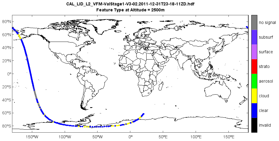
CALIPSO data

NASA launched the CloudSat and the Cloud-Aerosol Lidar and Infrared Pathfinder Satellite Observation (CALIPSO) spacecraft to study the role that clouds and aerosols play in regulating Earth’s weather, climate and air quality. On April 28, 2006. This example illustrates how to access and visualize a LaRC CALIPSO data file.

# Add file
fn = 'CAL_LID_L2_VFM-ValStage1-V3-02.2011-12-31T23-18-11ZD.hdf'
f = addfile('D:/Temp/hdf/' + fn)

# Read data
vname = 'Feature_Classification_Flags'
var = f[vname]
data = var[:,1256]
lon = f['Longitude'][:,0]
lat = f['Latitude'][:,0]
lon = lon[::10]
lat = lat[::10]
data = data[::10]

# Extract Feature Type only through bitmask.
data = data & 7

# Plot
axesm()
geoshow('country', edgecolor='k')
levs = arange(8)
cols = [(0,0,0),(0,0,255),(255,255,0),(0,255,0),(255,0,0), \
    (200,100,255),(100,50,255),(127,127,127)]
ls = makesymbolspec('point', levels=levs, colors=cols)
layer = scatter(lon, lat, data, size=5, edge=False, symbolspec=ls)
colorbar(layer, ticklabels=['invalid', 'clear', 'cloud', 'aerosol', \
    'strato', 'surface', 'subsurf', 'no signal'])
xlim(-180, 180)
ylim(-90, 90)
title([fn, 'Feature Type at Altitude = 2500m'])

# Add file
fn = 'D:/Temp/hdf/CAL_LID_L2_VFM-ValStage1-V3-02.2011-12-31T23-18-11ZD.hdf'
f = addfile(fn)

# Read data
vname = 'Feature_Classification_Flags'
var = f[vname]
data = var[:,:]
lat = f['Latitude'][:,0]

# Extract Feature Type only through bitmask.
data = data & 7

# Subset latitude values for the region of interest (40N to 62N).
lat = lat[3500:4000]
size = lat.shape[0]

data2d = data[3500:4000, 1165:]  # -0.5km to  8.2km
data3d = reshape(data2d, (size, 15, 290))
data = data3d[:,0,:]

# Focus on cloud (=2) data only.
data[data > 2] = 0
data[data < 2] = 0
data[data == 2] = 1

# Generate altitude data according to file specification [1].
alt = zeros(290)
# -0.5km to 8.2km
for i in range (0, 290):
    alt[i] = -0.5 + i*0.03

# Plot
levs = arange(2)
cols = ['w','b']
ls = makesymbolspec('image', levels=levs, colors=cols)
layer = imshow(rot90(data, 3), symbolspec=ls, extent=[lat[0],lat[-1],alt[0],alt[-1]])
colorbar(layer, ticklabels=['Others','Cloud'])
basename = os.path.basename(fn)
title([basename, 'Feature Type (Bits 1-3) in Feature Classification Flag'])
xlabel('Latitude (degrees north)')
ylabel('Altitude (km)')

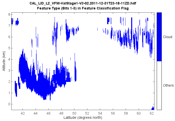
Vertical feature types.

# Add file
fn = 'D:/Temp/hdf/CAL_LID_L2_VFM-Standard-V4-10.2013-12-08T04-46-10ZD.hdf'
f = addfile(fn)

# Read data
vname = 'Feature_Classification_Flags'
var = f[vname]
data = var[:,:]
lat = f['Latitude'][:,0]

# Extract Feature Type only through bitmask.
data = data & 7

# Subset latitude values for the region of interest (40N to 62N).
lat = lat[3000:4000]
size = lat.shape[0]

data2d = data[3000:4000, 1165:]  # -0.5km to  8.2km
data3d = reshape(data2d, (size, 15, 290))
data = data3d[:,0,:]

# Generate altitude data according to file specification [1].
alt = zeros(290)
# -0.5km to 8.2km
for i in range (0, 290):
    alt[i] = -0.5 + i*0.03

# Plot
levs = arange(8)
cols = [(255,255,255),(0,0,255),(51,255,255),(255,153,0),(255,255,0),(0,255,0),(127,127,127),(0,0,0)]
ls = makesymbolspec('image', levels=levs, colors=cols)
layer = imshow(rot90(data, 1), symbolspec=ls, extent=[lat[0],lat[-1],alt[0],alt[-1]])
colorbar(layer, ticklabels=['Invalid', 'Clear Air', 'Cloud', 'Aerosol', 'Strato Feature', 'Surface', 'Subsurface', 'No Signal'])
basename = os.path.basename(fn)
title([basename, 'Feature Type (Bits 1-3) in Feature Classification Flag'])
xlabel('Latitude (degrees north)')
ylabel('Altitude (km)')
xaxis(tickin=False)
yaxis(tickin=False)

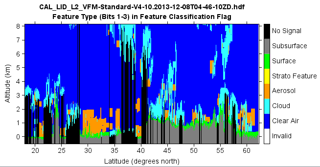
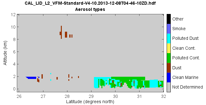
Aerosol types.

# Add file
fn = 'D:/Temp/hdf/CAL_LID_L2_VFM-Standard-V4-10.2013-12-08T04-46-10ZD.hdf'
f = addfile(fn)

# Read data
vname = 'Feature_Classification_Flags'
var = f[vname]
data = var[:,:]
lat = f['Latitude'][:,0]
lon = f['Longitude'][:,0]

# Subset latitude values for the region of interest.
lidx1 = 3176
lidx2 = 3313
lat = lat[lidx1:lidx2]
lon = lon[lidx1:lidx2]
size = lat.shape[0]

N = 290    # 290 is sample numbe of low hight data: -0.5km to 8.2km
sidx = data.shape[1] - N * 15
data2d = data[lidx1:lidx2, sidx:]
data3d = reshape(data2d, (size, 15, N))
data_l = data3d[:,0,:]
#data_l = rot90(data_1, 1)

sidx1 = sidx - 200 * 5
data2d = data[lidx1:lidx2, sidx1:sidx]
data3d = reshape(data2d, (size, 5, 200))
data_m = data3d[:,0,:]
data_m1 = zeros([data_m.shape[0], data_m.shape[1]*2])
for i in range(data_m.shape[1]):
    data_m1[:,i*2] = data_m[:,i]
    data_m1[:,i*2+1] = data_m[:,i]
#data_m = rot90(data_1, 1)

data = concatenate([data_m1, data_l], axis=1)
data = rot90(data, 1)

# Aerosol type
a = data >> 9
temp = a & 7
type2 = data & 7
tmask = (type2 == 3)
temp1 = (temp!=0)
temp2 = (temp1 & tmask)
atype = temp * temp2

# Generate altitude data according to file specification [1].
alt = zeros(N + 200*2)
# -0.5km to 20.2km
for i in range (0, N+200*2):
    alt[i] = -0.5 + i * 0.03

# Plot
levs = arange(8)
cols = [(204,204,204),(0,0,255),(153,51,0),(0,204,0),(255,241,85),(0,255,255),\
    (102,102,255),(0,0,0)]
ls = makesymbolspec('image', levels=levs, colors=cols)
layer = imshow(atype, symbolspec=ls, extent=[lat[0],lat[-1],alt[0],alt[-1])
colorbar(layer, ticklabels=['Not Determined','Clean Marine','Dust','Polluted Cont.','Clean Cont.',\
    'Polluted Dust','Smoke','Other'])
basename = os.path.basename(fn)
title([basename, 'Aerosol types'])
xlabel('Latitude (degrees north)')
ylabel('Altitude (km)')
ylim(-0.5, 12.1)

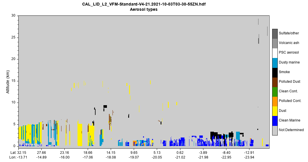
Aerosol types of tropospheric and stratospheric aerosols.

# Add file
fn = 'D:/Temp/hdf/CAL_LID_L2_VFM-Standard-V4-21.2021-10-03T03-30-55ZN.hdf'
f = addfile(fn)

# Read data
vname = 'Feature_Classification_Flags'
var = f[vname]
data = var[:,:]
lat = f['Latitude'][:,0]
lon = f['Longitude'][:,0]

# Subset latitude values for the region of interest.
lidx1 = 1088
lidx2 = 2175
lat = lat[lidx1:lidx2]
lon = lon[lidx1:lidx2]
size = lat.shape[0]

N = 290    # 290 is sample number of low height data: -0.5km to 8.2km @ 30m
sidx = data.shape[1] - N * 15
data2d = data[lidx1:lidx2, sidx:]
data3d = reshape(data2d, (size, 15, N))
data_l = data3d[:,0,:]

N1 = 200   # height data: 8.2 to 20.2 km @ 60m
sidx1 = sidx - N1 * 5
data2d = data[lidx1:lidx2, sidx1:sidx]
data3d = reshape(data2d, (size, 5, N1))
data_m = data3d[:,0,:]
data_m1 = zeros([data_m.shape[0], data_m.shape[1]*2], dtype='int')
data_m1[:,::2] = data_m
data_m1[:,1::2] = data_m

N2 = 55   # height data: 20.2 to 30.1km @ 180m
sidx2 = sidx1 - N2 * 3
data2d = data[lidx1:lidx2, sidx2:sidx1]
data3d = reshape(data2d, (size, 3, N2))
data_m = data3d[:,0,:]
data_m2 = zeros([data_m.shape[0], data_m.shape[1]*6], dtype='int')
for i in range(6):
    data_m2[:,i::6] = data_m

data = concatenate([data_m2, data_m1, data_l], axis=1)
data = rot90(data, 1)

# Feature type
ft = data & 7

# Aerosol type
a = data >> 9
# tropospheric aerosol
atype = a & 7
atype[ft!=3] = 0
# stratospheric aerosol
btype = a & 7
btype[ft!=4] = 0
# combin
btype = btype + 8
btype[btype==8] = 0
btype[btype>3+8] = 0
#atype[btype>0] = 0
atype = atype + btype

# Generate altitude data according to file specification [1].
alt = zeros(N + N1 * 2 + N2 * 6)
# -0.5km to 30.1km
for i in range (0, N + N1 * 2 + N2 * 6):
    alt[i] = -0.5 + i * 0.03

# X axis ticks
xvals = []
xstrs = []
nx = atype.shape[1]
for i in range(0, nx, 100):
    xvals.append(i)
    if i == 0:
        xstrs.append('Lat: %.2f\nLon: %.2f' % (lat[i],lon[i]))
    else:
        xstrs.append('%.2f\n%.2f' % (lat[i],lon[i]))

# Plot
axes(tickfontsize=12)
levs = arange(11)
cols = [(204,204,204),(0,0,255),(255,240,0),(255,153,0),(51,153,0),
    (120,51,0),'k',(0,153,204),'w',(150,150,150),(100,100,100)]
imshow(atype, levs, colors=cols, extent=[0,nx-1,alt[0],alt[-1]])
colorbar(shrink=0.8, fontsize=12, ticklabels=['Not Determined','Clean Marine',
    'Dust','Polluted Cont.','Clean Cont.','Polluted Dust','Smoke',
    'Dusty marine','PSC aerosol','Volcanic ash','Sulfate/other'])
xticks(xvals, xstrs)
yaxis(minortick=True)
basename = os.path.basename(fn)
title([basename, 'Aerosol types'])
ylabel('Altitude (km)')
ylim(-0.5, 30.1)

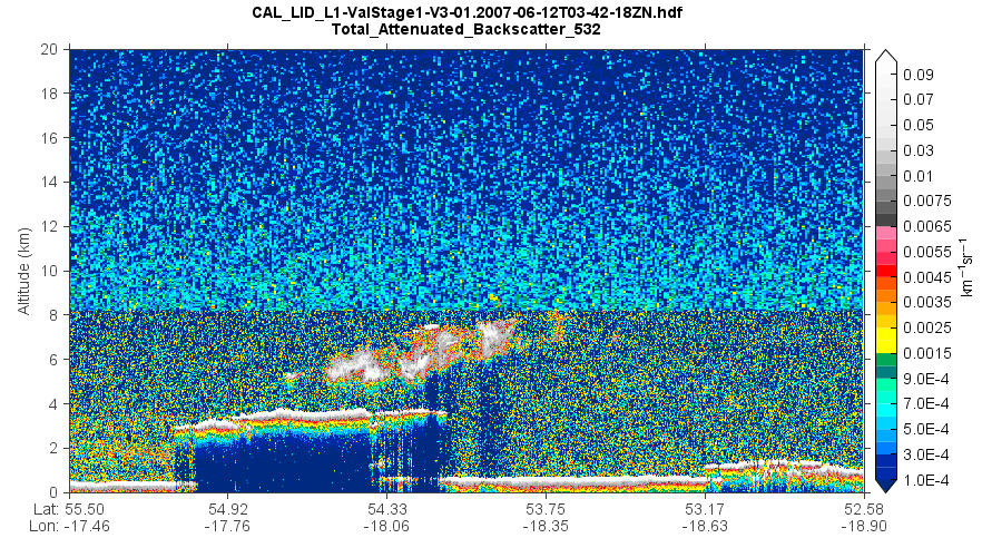
Plot total attenuated backscatter.

# Add file
fn = 'D:/Temp/hdf/CAL_LID_L1-ValStage1-V3-01.2007-06-12T03-42-18ZN.hdf'
f = addfile(fn)

# Read data
x1 = 0
x2 = 1001
nx = x2 - x1
h1 = 0  # km
h2 = 20  # km
nz = 500  # Number of pixels in the vertical
vname = 'Total_Attenuated_Backscatter_532'
var = f[vname]
data = var[x1:x2,:]
data = rot90(data)
lats = f['Latitude'][x1:x2,0]
lons = f['Longitude'][x1:x2,0]
height = f['metadata']['Lidar_Data_Altitudes']
height = height[::-1]
data.setdimvalue(0, height)

# Interpolate data on a regular grid
x = arange(x1, x2)
h = linspace(h1, h2, nz)
data = interpolate.linint2(data, x, h)

# X axis ticks
xvals = []
xstrs = []
for i in range(0, nx, 200):
    xvals.append(i + x1)
    if i == 0:
        xstrs.append('Lat: %.2f\nLon: %.2f' % (lats[i],lons[i]))
    else:
        xstrs.append('%.2f\n%.2f' % (lats[i],lons[i]))

# Plot
levs = [0.0001,0.0002,0.0003,0.0004,0.0005,0.0006,0.0007,0.0008,0.0009,
    0.001,0.0015,0.002,0.0025,0.003,0.0035,0.004,0.0045,0.005,0.0055,0.006,
    0.0065,0.007,0.0075,0.008,0.01,0.02,0.03,0.04,0.05,0.06,0.07,0.08,0.09,0.1]
layer = imshow(x, h, data, levs, cmap='calipo_standard', interpolation='bilinear')
xaxis(tickin=False)
yaxis(tickin=False)
xticks(xvals, xstrs)
ylabel('Altitude (km)')
colorbar(layer, extendrect=False, label=r'$\rm{km}^{-1} \rm{sr}^{-1}$')
basename = os.path.basename(fn)
title('{0}\n{1}'.format(basename, vname))

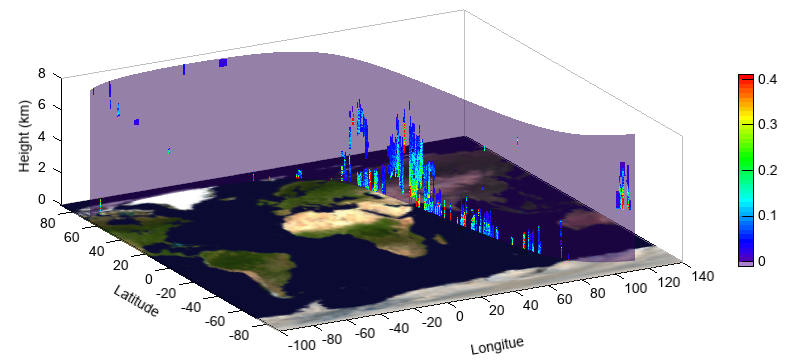
Plot 3D cross section of extinction coefficient.

f = addfile('D:/Temp/satellite/calipso/CAL_LID_L2_05kmAPro-Standard-V4-20.2006-09-01T08-55-57ZD_Subset.hdf')
EC = f['Extinction_Coefficient_532'][:]
EC = rot90(EC, 1)
EC[EC==nan] = -1
Lat = f['Latitude'][:,0]
Lon = f['Longitude'][:,0]

alt1 = arange(-0.5,20.08,0.06).tolist()
alt2 = arange1(20.2,56,0.18).tolist()
alt = array(alt1 + alt2)

Lon = Lon[np.newaxis,:]
Lon = Lon.repeat(len(alt),0)
Lat = Lat[np.newaxis,:]
Lat = Lat.repeat(len(alt),0)
alt = alt[:,np.newaxis]
alt = alt.repeat(Lon.shape[1],1)

fn = os.path.join(migl.get_map_folder(), 'world_topo.jpg')
land = georead(fn)

#plot
levs = arange(0,0.41,0.01)
cols = makecolors(len(levs)+1, cmap='rainbow')
cols[0] = miutil.getcolor(cols[0], alpha=0.5)
ax = axes3d()
grid(False)
#lighting()
geoshow(land)
surf(Lon[::10,::10], Lat[::10,::10], alt[::10,::10], levs, colors=cols,
    facecolor='texturemap', cdata=EC, edgecolor=None)
colorbar(aspect=30, ticks=[0,0.1,0.2,0.3,0.4,0.5])
zlim(0,8)
xlim(-100,140)
ylim(-90,90)
xlabel('Longitue')
ylabel('Latitude')
zlabel('Height (km)')

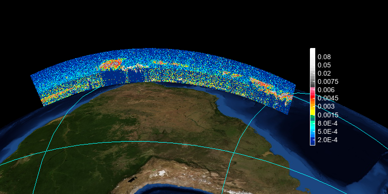
Plot total attenuated backscatter in earth 3D axes.

# Add file
fn = 'D:/Temp/hdf/CAL_LID_L1-ValStage1-V3-01.2007-06-12T03-42-18ZN.hdf'
f = addfile(fn)

# Read data
x1 = 15000
x2 = 30001
nx = x2 - x1
h1 = 0  # km
h2 = 20  # km
nz = 500  # Number of pixels in the vertical
vname = 'Total_Attenuated_Backscatter_532'
var = f[vname]
data = var[x1:x2,:]
data = rot90(data)
Lat = f['Latitude'][x1:x2,0]
Lon = f['Longitude'][x1:x2,0]
alt = f['metadata']['Lidar_Data_Altitudes']
alt = alt[::-1]

# Interpolate data on a regular grid
x = arange(x1, x2)
h = linspace(h1, h2, nz)
data = interpolate.linint2(x, alt, data, x, h)

Lon = Lon[np.newaxis,:]
Lon = Lon.repeat(nz,0)
Lat = Lat[np.newaxis,:]
Lat = Lat.repeat(nz,0)
alt = h[:,np.newaxis]
alt = alt.repeat(Lon.shape[1],1)

# Plot
ax = axes3d(earth=True)
ax.lonlat(color='c')
levs = [0.0001,0.0002,0.0003,0.0004,0.0005,0.0006,0.0007,0.0008,0.0009,
    0.001,0.0015,0.002,0.0025,0.003,0.0035,0.004,0.0045,0.005,0.0055,0.006,
    0.0065,0.007,0.0075,0.008,0.01,0.02,0.03,0.04,0.05,0.06,0.07,0.08,0.09,0.1]
ss = 20
surf(Lon[::ss,::ss], Lat[::ss,::ss], alt[::ss,::ss]*30, levs,
    facecolor='texturemap', cdata=data, edgecolor=None,
    cmap='calipo_standard', interpolation='bilinear')

ax.set_rotation(333)
ax.set_elevation(-47)
ax.set_head(270)
ax.set_pitch(-90)

v = 820
axis([-v,v,-v,v,-v,v])

colorbar(tickcolor='w', xshift=80)