GEOS-16 data

This example code illustrates how to access and visualize a GEOS-16 data.

fn = 'D:/Temp/nc/OR_ABI-L1b-RadC-M4C02_G16_s20161811455312_e20161811500122_c20161811500164.nc'
f = addfile(fn)
rad = f['Rad'][::-1,:]
rad[rad>800] = nan
x = f['x'][:]
y = f['y'][::-1]
geos_p = f['goes_imager_projection']
proj_name = geos_p.attrvalue('grid_mapping_name')[0]
h = geos_p.attrvalue('perspective_point_height')[0]
a = geos_p.attrvalue('semi_major_axis')[0]
b = geos_p.attrvalue('semi_minor_axis')[0]
rf = geos_p.attrvalue('inverse_flattening')[0]
lat_0 = geos_p.attrvalue('latitude_of_projection_origin')[0]
lon_0 = geos_p.attrvalue('longitude_of_projection_origin')[0]
sweep = geos_p.attrvalue('sweep_angle_axis')[0]
pstr = '+proj=geos +h=%f +a=%f +b=%f +rf=%f +lat_0=%f +lon_0=%f' \
    % (h, a, b, rf, lat_0, lon_0)

#Following the simple formula for the projection coordinate,
#proj_coor = scan_angle_radians * height
x = x * h
y = y * h

#Project
proj = projinfo(proj4string=pstr)

#Plot
axesm(projinfo=proj, gridline=True)
geoshow('country', edgecolor='k')
ls = imshow(x, y, rad, 40, proj=proj)
colorbar(ls)
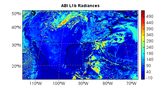
title('ABI L1b Radiances')