SeaWiFS grid data

This example code illustrates how to access and visualize a SeaWiFS grid data.

#Add data file
f = addfile('D:/Temp/hdf/S1999001.L3m_DAY_CHL_chlor_a_9km.hdf')
#Get data variable
vname = 'l3m_data'
v = f[vname]
#Set x/y
ny = f.attrvalue('Number_of_Lines')[0]
nx = f.attrvalue('Number_of_Columns')[0]
sx = f.attrvalue('Westernmost_Longitude')[0]
ex = f.attrvalue('Easternmost_Longitude')[0]
sy = f.attrvalue('Southernmost_Latitude')[0]
ey = f.attrvalue('Northernmost_Latitude')[0]
x = linspace(sx, ex, nx)
y = linspace(sy, ey, ny)
#Set x/y dimensions
v.setdim('Y', y, 0)
v.setdim('X', x, 1)
#Get data array
fillv = v.attrvalue('Fill')[0]
scale = v.attrvalue('Slope')[0]
offset = v.attrvalue('Intercept')[0]
data = v[::-1,:] * scale + offset
data.fill_value = fillv
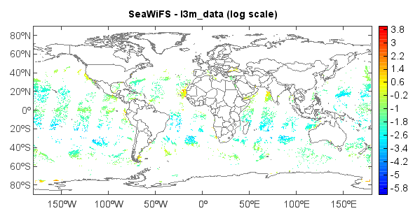
data = log(data)
#Plot
axesm()
geoshow('country')
levs = arange(-6, 4, 0.2)
layer = imshow(data, levs)
colorbar(layer)
title('SeaWiFS - ' + vname + ' (log scale)')