Fisher’s linear discriminant

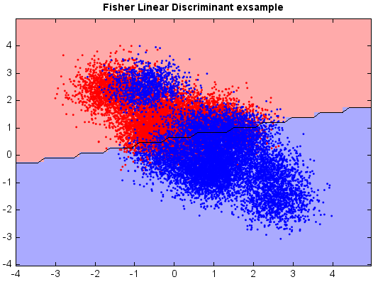
Fisher’s linear discriminant (FLD) is another popular linear classifier. Fisher defined the separation between two distributions to be the ratio of the variance between the classes to the variance within the classes, which is, in some sense, a measure of the signal-to-noise ratio for the class labeling. FLD finds a linear combination of features which maximizes the separation after the projection. The resulting combination may be used for dimensionality reduction before later classification.

from miml import datasets
from miml.classification import FisherLinearDiscriminant

fn = os.path.join(datasets.get_data_home(), 'classification', 'toy',
    'toy-test.txt')
df = DataFrame.read_table(fn, header=None, names=['x1','x2'],
    format='%2f', index_col=0)

X = df.values
y = array(df.index.data)

model = FisherLinearDiscriminant()
model.fit(X, y)

# Plot the decision boundary. For that, we will assign a color to each
# point in the mesh [x_min, x_max]x[y_min, y_max].
x_min, x_max = X[:, 0].min() - 1, X[:, 0].max() + 1
y_min, y_max = X[:, 1].min() - 1, X[:, 1].max() + 1
n = 50  # size in the mesh
xx, yy = np.meshgrid(np.linspace(x_min, x_max, n),
                     np.linspace(y_min, y_max, n))
data = np.vstack((xx.flatten(), yy.flatten())).T
Z = model.predict(data)

# Put the result into a color plot
Z = Z.reshape(xx.shape)

#Plot
# Create color maps
cmap_light = ['#FFAAAA', '#AAAAFF']
cmap_bold = ['#FF0000', '#0000FF']
imshow(xx[0,:], yy[:,0], Z, colors=cmap_light)
# Plot also the training points
ls = plt.scatter(X[:, 0], X[:, 1], c=y,
            edgecolor=None, s=3, levels=[0,1], colors=cmap_bold)
plt.contour(xx[0,:], yy[:,0], Z, [0.5], color='k', smooth=False)
plt.xlim(xx.min(), xx.max())
plt.ylim(yy.min(), yy.max())
plt.title("Fisher Linear Discriminant exsample")