Linear discriminant analysis

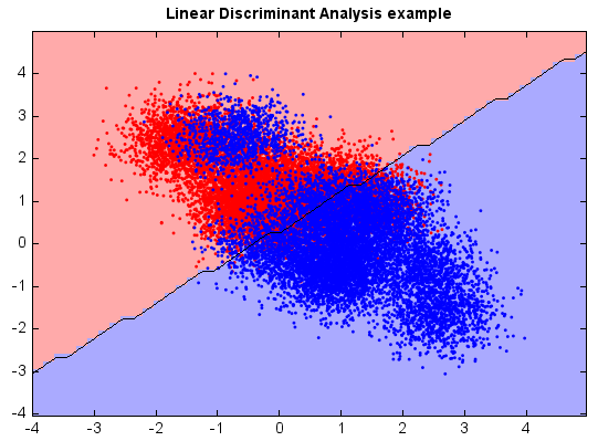
Linear discriminant analysis (LDA) is based on the Bayes decision theory and assumes that the conditional probability density functions are normally distributed. LDA also makes the simplifying homoscedastic assumption (i.e. that the class covariances are identical) and that the covariances have full rank. With these assumptions, the discriminant function of an input being in a class is purely a function of this linear combination of independent variables.

from miml import datasets
from miml.classification import LinearDiscriminantAnalysis

fn = os.path.join(datasets.get_data_home(), 'classification', 'toy',
    'toy-test.txt')
df = DataFrame.read_table(fn, header=None, names=['x1','x2'],
    format='%2f', index_col=0)

X = df.values
y = array(df.index.data)

model = LinearDiscriminantAnalysis()
model.fit(X, y)

# Plot the decision boundary. For that, we will assign a color to each
# point in the mesh [x_min, x_max]x[y_min, y_max].
x_min, x_max = X[:, 0].min() - 1, X[:, 0].max() + 1
y_min, y_max = X[:, 1].min() - 1, X[:, 1].max() + 1
n = 50  # size in the mesh
xx, yy = np.meshgrid(np.linspace(x_min, x_max, n),
                     np.linspace(y_min, y_max, n))
data = np.vstack((xx.flatten(), yy.flatten())).T
Z = model.predict(data)

# Put the result into a color plot
Z = Z.reshape(xx.shape)

#Plot
# Create color maps
cmap_light = ['#FFAAAA', '#AAAAFF']
cmap_bold = ['#FF0000', '#0000FF']
imshow(xx[0,:], yy[:,0], Z, colors=cmap_light)
# Plot also the training points
ls = plt.scatter(X[:, 0], X[:, 1], c=y,
            edgecolor=None, s=3, levels=[0,1], colors=cmap_bold)
plt.contour(xx[0,:], yy[:,0], Z, [0.5], color='k', smooth=False)
plt.xlim(xx.min(), xx.max())
plt.ylim(yy.min(), yy.max())
plt.title("Linear Discriminant Analysis example")