K-Nearest Neighbor

The k-nearest neighbor algorithm (k-NN) is a method for classifying objects by a majority vote of its neighbors, with the object being assigned to the class most common amongst its k nearest neighbors (k is typically small). k-NN is a type of instance-based learning, or lazy learning where the function is only approximated locally and all computation is deferred until classification.

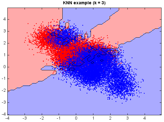
Nearest neighbor rules in effect compute the decision boundary in an implicit manner. In the following example, we show the implicit decision boundary of k-NN on a 2-dimensional toy data. Please try different k, and you will observe the change of decision boundary. In general, the larger k, the smoother the boundary.

from miml import datasets
from miml.classification import KNearestNeighbor

fn = os.path.join(datasets.get_data_home(), 'classification', 'toy',
    'toy-test.txt')
df = DataFrame.read_table(fn, header=None, names=['x1','x2'],
    format='%2f', index_col=0)

X = df.values
y = array(df.index.data)

n_neighbors = 3
knn = KNearestNeighbor(n_neighbors)
knn.fit(X, y)

# Plot the decision boundary. For that, we will assign a color to each
# point in the mesh [x_min, x_max]x[y_min, y_max].
x_min, x_max = X[:, 0].min() - 1, X[:, 0].max() + 1
y_min, y_max = X[:, 1].min() - 1, X[:, 1].max() + 1
n = 50  # size in the mesh
xx, yy = np.meshgrid(np.linspace(x_min, x_max, n),
                     np.linspace(y_min, y_max, n))
data = np.vstack((xx.flatten(), yy.flatten())).T
Z = knn.predict(data)

# Put the result into a color plot
Z = Z.reshape(xx.shape)

#Plot
# Create color maps
cmap_light = ['#FFAAAA', '#AAAAFF']
cmap_bold = ['#FF0000', '#0000FF']
imshow(xx[0,:], yy[:,0], Z, colors=cmap_light)
# Plot also the training points
ls = plt.scatter(X[:, 0], X[:, 1], c=y,
            edgecolor=None, s=3, levels=[0,1], colors=cmap_bold)
plt.contour(xx[0,:], yy[:,0], Z, [0.5], color='k', smooth=False)
plt.xlim(xx.min(), xx.max())
plt.ylim(yy.min(), yy.max())
plt.title("KNN example (k = %i)"
          % (n_neighbors))

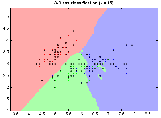
3-class classification:

from miml import datasets
from miml.classification import KNearestNeighbor

iris = datasets.load_iris()

# we only take the first two features. We could avoid this ugly
# slicing by using a two-dim dataset
X = iris.data[:, :2]
y = iris.target

n_neighbors = 15
model = KNearestNeighbor(n_neighbors)
model.fit(X, y)

# Plot the decision boundary. For that, we will assign a color to each
# point in the mesh [x_min, x_max]x[y_min, y_max].
x_min, x_max = X[:, 0].min() - 1, X[:, 0].max() + 1
y_min, y_max = X[:, 1].min() - 1, X[:, 1].max() + 1
h = .02  # step size in the mesh
xx, yy = np.meshgrid(np.arange(x_min, x_max, h),
                     np.arange(y_min, y_max, h))
data = np.vstack((xx.flatten(), yy.flatten())).T
Z = model.predict(data)

# Put the result into a color plot
Z = Z.reshape(xx.shape)

#Plot
# Create color maps
cmap_light = ['#FFAAAA', '#AAFFAA', '#AAAAFF']
cmap_bold = ['#FF0000', '#00FF00', '#0000FF']
pcolor(xx, yy, Z, colors=cmap_light)
# Plot also the training points
ls = plt.scatter(X[:, 0], X[:, 1], c=y,
            edgecolor='k', s=4, levels=[0,1,2], colors=cmap_bold)
plt.xlim(xx.min(), xx.max())
plt.ylim(yy.min(), yy.max())
plt.title("3-Class classification (k = %i)"
          % (n_neighbors))