MeteoInfo 4.2.0 was released (2026-3-21)
Add loc and sel functions in DimVariable and DimArray classes for selecting data using label-based indexing
Including new developed symjy toolbox for symbol calculation
Add lifted_index and precipitable_water functions in meteolib package
Add cross function in linalg package
Add clip, bitwise_and, bitwise_or and bitwise_xor functions in numeric.core package
Add faces and vertices data support in patch plot function
Add PolyCollection class in plotlib package
Support micaps mdfs 125 type data file
Improve slice3 function to support 2D data array
Improve geotiff data reading for predictor tag
Update FlatlLaf to version 3.6.1
Update JOGL to version 2.6.0
Some bug fixed
select data with sel function
fn = 'D:/Temp/nc/sst.mon.anom.nc'
f = addfile(fn)
print(f.time[0])
dt = f.dims.time.dt
syear = 1979; eyear = 2020
tidx = (dt.year >= syear) & (dt.year <= eyear) & (dt.month == 1)
sst = f.sst.sel(time=tidx, lat=slice(-30,30), lon=slice(160,300))
lats = f.lat.sel(lat=slice(-30,30))
lons = f.lon.sel(lon=slice(160,300))
# Create an EOF solver to do the EOF analysis. Square-root of cosine of
# latitude weights are applied before the computation of EOFs.
coslat = np.cos(np.deg2rad(lats))
wgts = np.sqrt(coslat)[..., np.newaxis]
solver = meteolib.EOF(sst, weights=wgts)
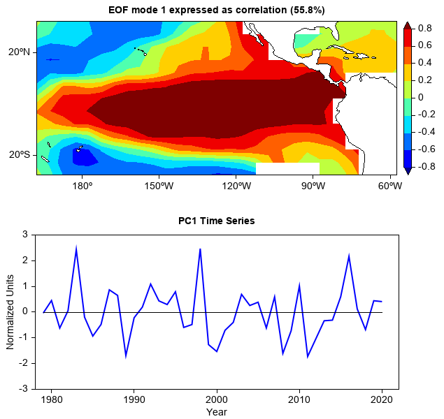
# Retrieve the leading EOF, expressed as the correlation between the leading
# PC time series and the input SST anomalies at each grid point, and the
# leading PC time series itself.
eof1 = solver.eofs_correlation(neofs=1)
pc1 = solver.pcs(npcs=1, pcscaling=1)
e1 = solver.variance_fraction(1)[0]
#Plot
subplot(2,1,1,axestype='map')
geoshow('continent', facecolor='w')
levs = arange(-0.8, 1, 0.2)
layer = contourf(lons, lats, eof1.squeeze(), levs, extend='both',
cmap='matlab_jet', smooth=False, zorder=0)
yticks(arange(-20, 61, 40))
colorbar(layer)
title('EOF mode 1 expressed as correlation (%.1f%%)' % (e1*100))
subplot(2,1,2)
years = range(syear, eyear+1)
lines = plot(years, pc1, color='b', linewidth=2, antialias=True)
y = zeros(len(years))
plot(years, y, color='k')
xlim(syear-1, eyear+1)
ylim(-3,3)
xticks(arange(1970,2021,10))
xlabel('Year')
ylabel('Normalized Units')
title('PC1 Time Series')
usage examples for symjy toolbox
from symjy import *

# Define symbols
x, y, z = symbols('x y z')
a, b, c = symbols('a b c', real=True)

# Basic examples
# Example 1: Basic symbolic expressions
expr1 = x**2 + 2*x + 1
print('Expression: {}'.format(expr1))
print("# Expected: x**2 + 2*x + 1")
print

# Example 2: Expansion
expr2 = (x + 1)**3
expanded = expand(expr2)
print("Expansion of (x+1)^3: {}".format(expanded))
print("# Expected: x**3 + 3*x**2 + 3*x + 1")
print

# Example 3: Factorization
expr3 = x**2 - 4
factored = factor(expr3)
print("Factorization of x^2 - 4: {}".format(factored))
print("# Expected: (x - 2)*(x + 2)")
print

# Example 4: Simplification
expr4 = (x**2 - 1)/(x - 1)
simplified = simplify(expr4)
print("Simplification of (x^2-1)/(x-1): {}".format(simplified))
print("# Expected: x + 1")
print

# Example 5: Partial fraction decomposition
expr5 = 1/(x**2 - 1)
partial_fractions = apart(expr5)
print("Partial fractions of 1/(x^2-1): {}".format(partial_fractions))
print("# Expected: -1/(2*(x + 1)) + 1/(2*(x - 1))")
print

# Example 6: Collect terms
expr6 = x**2 + 2*a*x + a**2 + 3*b*x + b
collected = collect(expr6, x)
print("Collect terms in x of {}:".format(expr6))
print("Result: {}".format(collected))
print("# Expected: x**2 + x*(2*a + 3*b) + a**2 + b")
print

# Calculus examples
# Example 1: Differentiation
f = x**3 + 2*x**2 + x + 1
df_dx = diff(f, x)
print("Derivative of {} w.r.t x: {}".format(f, df_dx))
print("# Expected: 3*x**2 + 4*x + 1")
print

# Example 2: Higher-order derivatives
d2f_dx2 = diff(f, x, 2)  # Second derivative
print("Second derivative of {}: {}".format(f, d2f_dx2))
print("# Expected: 6*x + 4")
print

# Example 3: Partial derivatives
g = x**2 * y + x * y**2
dg_dx = diff(g, x)
dg_dy = diff(g, y)
print("Function: {}".format(g))
print("Partial derivative w.r.t x: {}".format(dg_dx))
print("Partial derivative w.r.t y: {}".format(dg_dy))
print("# Expected: ∂g/∂x = 2*x*y + y**2, ∂g/∂y = x**2 + 2*x*y")
print

# Example 4: Integration
h = x**2 + 2*x + 1
integral = integrate(h, x)
print("Integral of {} w.r.t x: {}".format(h, integral))
print("# Expected: x**3/3 + x**2 + x")
print

# Example 5: Definite integration
definite_integral = integrate(h, (x, 0, 1))
print("Definite integral of {} from 0 to 1: {}".format(h, definite_integral))
print("# Expected: 7/3")
print

# Example 6: Limits
limit_expr = sin(x) / x
limit_result = limit(limit_expr, x, 0)
print("Limit of sin(x)/x as x->0: {}".format(limit_result))
print("# Expected: 1")
print

# Example 7: Series expansion
series_expansion = series(sin(x), x, 0, 6)  # 6 terms around x=0
print("Series expansion of sin(x) around 0: {}".format(series_expansion))
print("# Expected: x - x**3/6 + x**5/120 + O(x**6)")
print