volumeplot

Axes3DGL.volumeplot(*args, **kwargs):

creates a three-dimensional volume plot

Parameters:

• x – (array_like) Optional. X coordinate array.

• y – (array_like) Optional. Y coordinate array.

• z – (array_like) Optional. Z coordinate array.

• data – (array_like) 3D data array.

• cmap – (string) Color map string.

• vmin – (float) Minimum value for particle plotting.

• vmax – (float) Maximum value for particle plotting.

• ray_casting – (str) Ray casting algorithm [‘basic’ | ‘max_value’ | ‘specular’]. Default is ‘max_value’.

• brightness – (float) Volume brightness. Default is 1.

• alpha_min – (float) Minimum alpha value. Default is 0.

• alpha_max – (float) Maximum alpha value. Default is 1.

• opacity_nodes – (list of float) Opacity nodes. Default is None.

• opacity_levels – (list of float) Opacity levels. Default is [0., 1.].

Returns:

Volumeplot graphic

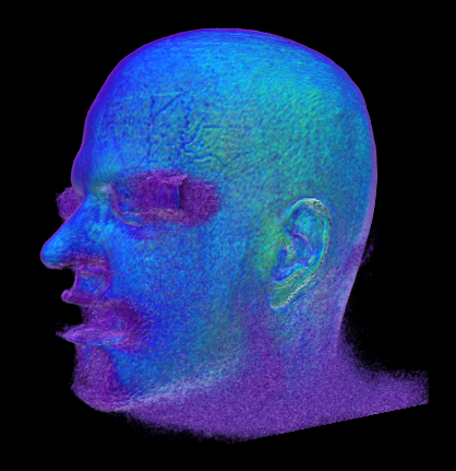
Example of 3D volume plot

fn = 'D:/Temp/image/sagittal.png'
data1 = imagelib.imread(fn)
data1 = data1[:,:,0]
data1 = data1.reshape(88,300,600)
data = zeros([176,300,300], dtype='int')
data[:88] = data1[::-1,:,:300]
data[88:] = data1[::-1,:,300:]
data = data.swapaxes(0, 1)

ax = axes3d(clip_plane=False)
ax.set_draw_box(False)
grid(False)
volumeplot(data, cmap='NCV_bright')

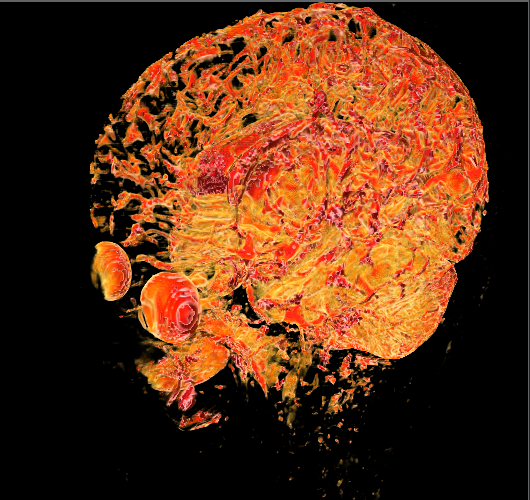
specular ray casting algorithm

fn = 'D:/Temp/image/sagittal.png'
data1 = imagelib.imread(fn)
data1 = data1[:,:,0]
data1 = data1.reshape(88,300,600)
data = zeros([176,300,300], dtype='int')
data[:88] = data1[::-1,:,:300]
data[88:] = data1[::-1,:,300:]
data = data.swapaxes(0, 1)

print('Plot...')
ax = axes3d(orthographic=False, aspect='equal', clip_plane=False,
    bgcolor='k', axis=False)
ax.set_draw_box(False)
grid(False)
volumeplot(data, cmap='MPL_sstanom', ray_casting='specular', brightness=1.5)

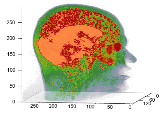
Set transfer function with opacity_nodes and opacity_levels arguments

fn = 'D:/Temp/image/sagittal.png'
data1 = imagelib.imread(fn)
data1 = data1[:,:,0]
data1 = data1.reshape(88,300,600)
data = zeros([176,300,300], dtype='int')
data[:88] = data1[::-1,:,:300]
data[88:] = data1[::-1,:,300:]
data = data.swapaxes(0, 1)

print('Plot...')
ax = axes3d(orthographic=False, aspect='equal', clip_plane=False,
    bgcolor='k', axis=False)
ax.set_draw_box(False)
grid(False)
volumeplot(data, cmap='MPL_sstanom', ray_casting='specular', brightness=1.5,
    opacity_nodes=[0,150,200,255], opacity_levels=[0,0,0.5,1])

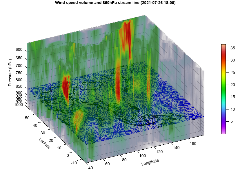
3D volume plot of temperature from numerical forecasting model of GRAPES

print('Read data...')
fn = 'D:/Temp/grib/grapes/rmf.tcgra.2021072500042.grb2'
f = addfile(fn)
tidx = 0
tt = f.gettime(tidx)
ss = 5
u = f['u-component_of_wind_isobaric'][tidx,::-1,::-ss,::ss]
v = f['v-component_of_wind_isobaric'][tidx,::-1,::-ss,::ss]
w = f['Vertical_velocity_geometric_isobaric'][tidx,::-1,::-ss,::ss]
u = u[:12]
v = v[:12]
w = w[:12]
speed = sqrt(u*u + v*v + w*w)
levels = u.dimvalue(0)
lat = u.dimvalue(1)
lon = v.dimvalue(2)
height = meteolib.pressure_to_height_std(levels * 0.01)

print('Plot...')
axes3d()
geoshow('country', edgecolor='k', edgesize=2, offset=height[5])
ss = 2
streamslice(lon[::ss], lat[::ss], height, u[:,::ss,::ss], v[:,::ss,::ss],
    w[:,::ss,::ss], zslice=[height[5]], color='b', density=2, interval=10, headwidth=0.2)
volumeplot(lon, lat, height, speed, cmap='NCV_bright')
colorbar(aspect=30)
zticks(height, (levels / 100).astype('int'))
xlabel('Longitude')
ylabel('Latitude')
zlabel('Pressure (hPa)')
xlim(lon[0], lon[-1])
ylim(lat[0], lat[-1])
title('Wind speed volume and 850hPa stream line ({})'.format(tt.strftime('%Y-%m-%d %H:00')))

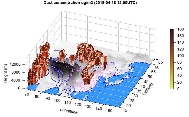
Using transfer function to simulate isosurface plot

#Set date
sdate = datetime.datetime(2019, 4, 15, 0)

#Set directory
datadir = 'D:/Temp/mm5'

#Read data
fn = os.path.join(datadir, 'WMO_SDS-WAS_Asian_Center_Model_Forecasting_CUACE-DUST_CMA_'+ sdate.strftime('%Y%m%d%H') + '.nc')
f = addfile(fn)
st = f.gettime(0)
t = 12
dust = f['CONC_DUST'][t,:,'15:65','65:155']
levels = dust.dimvalue(0)
dust[dust==nan] = 0
height = meteolib.pressure_to_height_std(levels)
lat = dust.dimvalue(1)
lon = dust.dimvalue(2)

#Relief data
rfn = 'D:/Temp/nc/elev.0.25-deg.nc'
rf = addfile(rfn)
elev = rf['data'][0,'15:65','65:155']
elev[elev<0] = -1
lon1 = elev.dimvalue(1)
lat1 = elev.dimvalue(0)
lon1, lat1 = meshgrid(lon1, lat1)

#Map
lchina = shaperead('cn_province')
clon = lchina.x_coord
clat = lchina.y_coord
calt = zeros(len(clon))
h = interp2d(elev, clon, clat)
calt = calt + h
lworld = shaperead('country')
wlon = lworld.x_coord
wlat = lworld.y_coord
walt = zeros(len(wlon))
h = interp2d(elev, wlon, wlat)
walt = walt + h

#Plot
ax = axes3d(clip_plane=False)
ax.set_elevation(-20)
ax.set_rotation(335)
rlevs = arange(0, 6000, 200)
cols = makecolors(len(rlevs) + 1, cmap='MPL_gist_yarg', alpha=1)
cols[0] = [51,153,255]
surf(lon1, lat1, elev, rlevs, facecolor='interp', colors=cols, edge=False)
plot3(clon, clat, calt, color=[255,153,255])
plot3(wlon, wlat, walt, color='b')
#Beijing location
plot3([116.39,116.39], [39.91,39.91], [0,12000])
pp = volumeplot(lon, lat, height, dust, ray_casting='specular',
    cmap='cmocean_solar_r', vmax=180, brightness=2.5,
    opacity_nodes=[90,100,120,121], opacity_levels=[0,0.5,0.5,0])
colorbar(pp, aspect=30)
xlim(65, 155)
xlabel('Longitude')
ylim(15, 65)
ylabel('Latitude')
zlim(0, 15000)
zlabel('Height (m)')
tt = st + datetime.timedelta(hours=t*3)
title('Dust concentration ug/m3 ({}UTC)'.format(tt.strftime('%Y-%m-%d %H:00')))