FY-2G cloud top temperature data

This example code illustrates how to access and visualize a FY-2G satellite cloud top temperature (CTT) data.

#Add data file
fn = 'D:/Temp/FY/FY2G_CTT_MLT_NOM_20180829_1200.hdf'
f = addfile(fn)

#Get data variable
ctt = f['CTT_Hourly_Product'][::-1]
ctt[ctt==0] = nan
nom = f['NomFileInfo']
clon = nom.member_array('NOMCenterLon')
sat_height = nom.member_array('NOMSatHeight')

#Set x/y
x = linspace(-5731466.255012655, 5726456.232062468, 2288)
y = linspace(-5726456.232062468, 5731466.255012655, 2288)

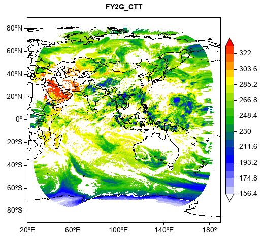
#Plot
ax = axesm(proj='geos', lon_0=clon, h=sat_height, gridlabel=False,
    frameon=False)
geoshow('country', edgecolor='k')
layer = imshow(x, y, ctt, 20, proj=ax.proj, cmap='wh-bl-gr-ye-re')
colorbar(layer, shrink=0.8, extendrect=False)
title('FY2G_CTT')

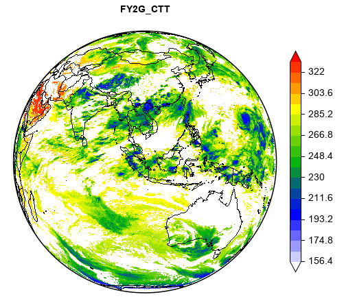
Project CTT data from geostationary projection to long/lat projection.

#Add data file
fn = 'D:/Temp/FY/FY2G_CTT_MLT_NOM_20180829_1200.hdf'
f = addfile(fn)

#Get data
ctt = f['CTT_Hourly_Product'][::-1]
ctt[ctt==0] = nan
nom = f['NomFileInfo']
clon = nom.member_array('NOMCenterLon')
sat_height = nom.member_array('NOMSatHeight')

#Set x/y
x = linspace(-5731466.255012655, 5726456.232062468, 2288)
y = linspace(-5726456.232062468, 5731466.255012655, 2288)

#Project data
fromproj = projinfo(proj='geos', lon_0=clon, h=sat_height)
toproj = projinfo()    #longlat projection
lon = arange(20, 190.1, 0.1)
lat = arange(-90, 90.1, 0.1)
ctt = geolib.reproject(ctt, x, y, fromproj, lon, lat, toproj)
londim = dimension(lon, 'lon', 'X')
latdim = dimension(lat, 'lat', 'Y')
ctt = DimArray(ctt, dims=[latdim, londim])

#Save projected data
ncwrite('D:/Temp/fy2g_proj.nc', ctt, 'ctt')

#Plot
ax = axesm()
geoshow('country')
layer = imshow(ctt, 20, cmap='wh-bl-gr-ye-re')
colorbar(layer, shrink=0.8, extendrect=False)
title('FY2G_CTT')